Reorder algorithms: Demand forecast

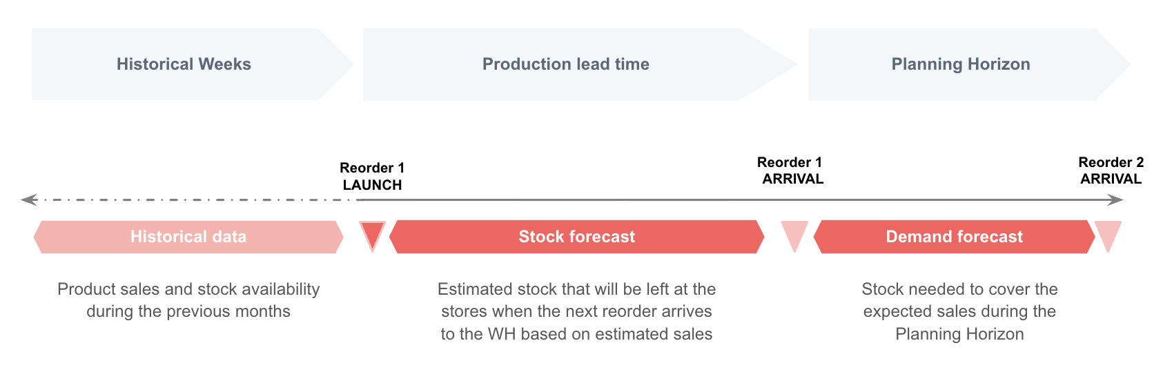
The demand forecast is built based on the sales data of the previous weeks.

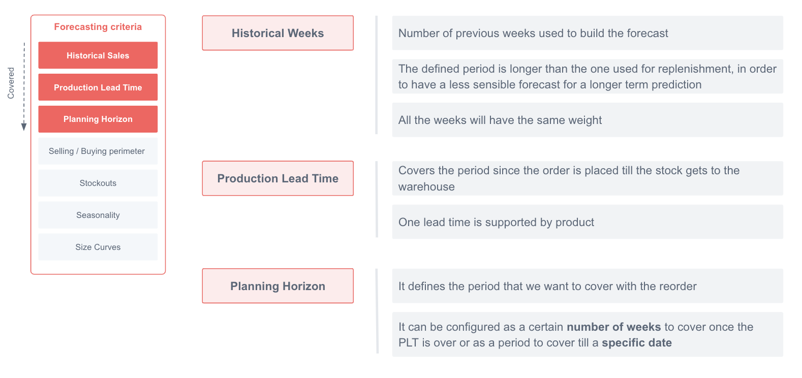
Demand forecast criteria: 

• Historical sales
• Production Lead Time
• Planning Horizon
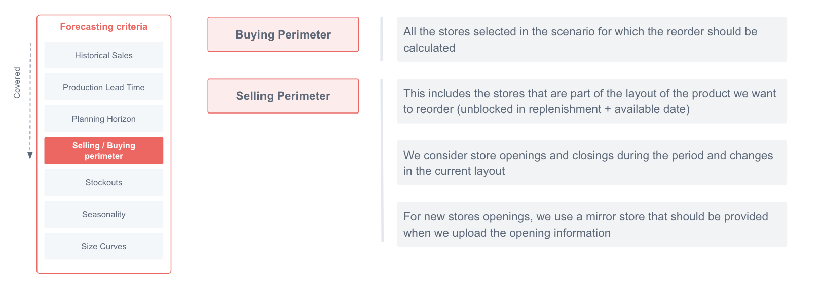
• Buying / Selling perimeter
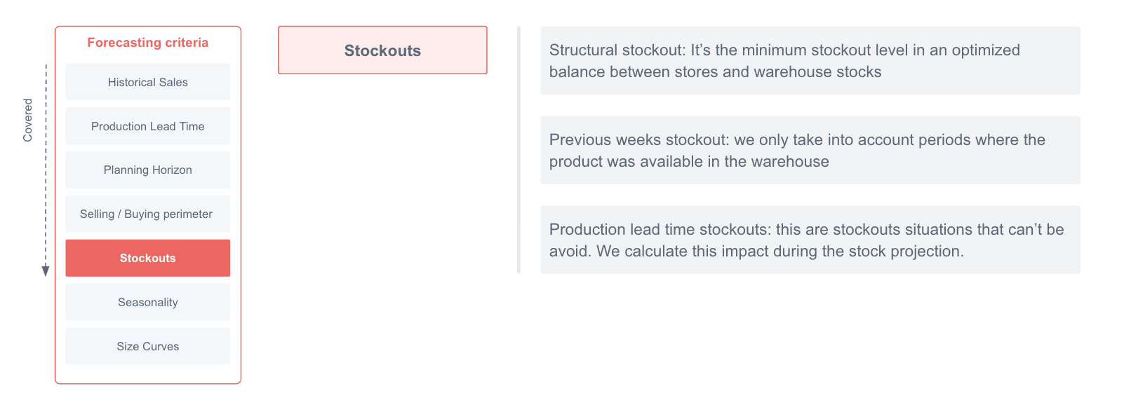
• Stockouts
• Seasonality
• Size Curves

The timeline of the Demand Forecast calculation is defined by the Historical weeks, the Lead Time, and the Planning Horizon.

Different store perimeters can be considered when calculating the forecast of each scenario

Out of stocks, both at the warehouse and at the stores, also play a role when estimating the reorder proposal

The effect in sales of recurring events is automatically taken into account by Nextail’s algorithms

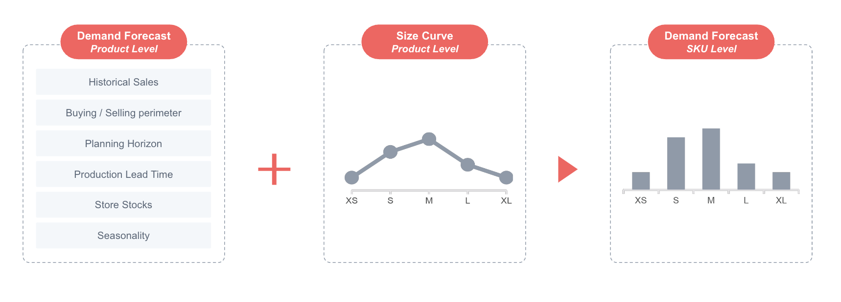
Size curves are recalculated in each scenario to break down to SKU level the Forecast obtained for each product

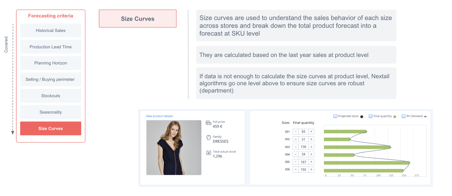
Once the demand forecast at product level has been calculated, the size curves are used to break it down and obtain a forecast by SKU

Promotions

Promotions are special events that have a temporary changing effect in a product’s demand during the time they are active. At this moment, promotions can be either markdowns or other kind of events.

Within Nextail framework, Promotions are expressed as a demand multiplicative factor called Promotions Coefficient. E.g. if there is a x2 promotions coefficient between two dates, some specific stores and products, it means demand (eventually sales) will be two times the usual ones.

The Promotions pipeline is in charge of retrieving and calculating the promotion coefficients for a group of products in a network of stores, at product-store-date level.

Customers are responsible for defining these coefficients for upcoming promotions they know will have an impact in demand. These are the future promotion coefficients. After the promotion period has ended, the defined coefficients are recalculated using true sales data to obtain what the real impact in demand was. These are the past promotion coefficients. Promotions have hence two effects in our forecast: 

1. Multiply the future demand that customers estimate by the future promotion coefficients. Let’s illustrate it:

• Customer estimates a x2 demand on product Random Sweater 101 within the second week of the year due to an special markdown.
• Forecast once applied seasonality is 200 SKUs within this week.
• A future promotion coefficient of 2 is applied, hence now 400 SKUs are the result of our forecast.

2. Correct (normalize) the sales data on which our forecast is trained, dividing them by past promotion coefficients.

• During the second week of the year, the customer finally sold 300 SKUs.
• Actual coefficient got is 300/200 = 0.5 (50%).
• For future forecasts we will take this 0.5 past promotion coefficient in order to normalize sales during sales period instead of using the original future promotion coefficient (which was 100%).

There’s a possibility where multiple promotions affects to the same product in the same stores and time period. In this cases only the max coefficient is taken into account.

Past availability

The past availability information provides a file with the day-store-product combinations where a product is available in the historical data used for the forecast. The importance of informing correctly the availability of a product allows us to estimate the demand instead of sales.

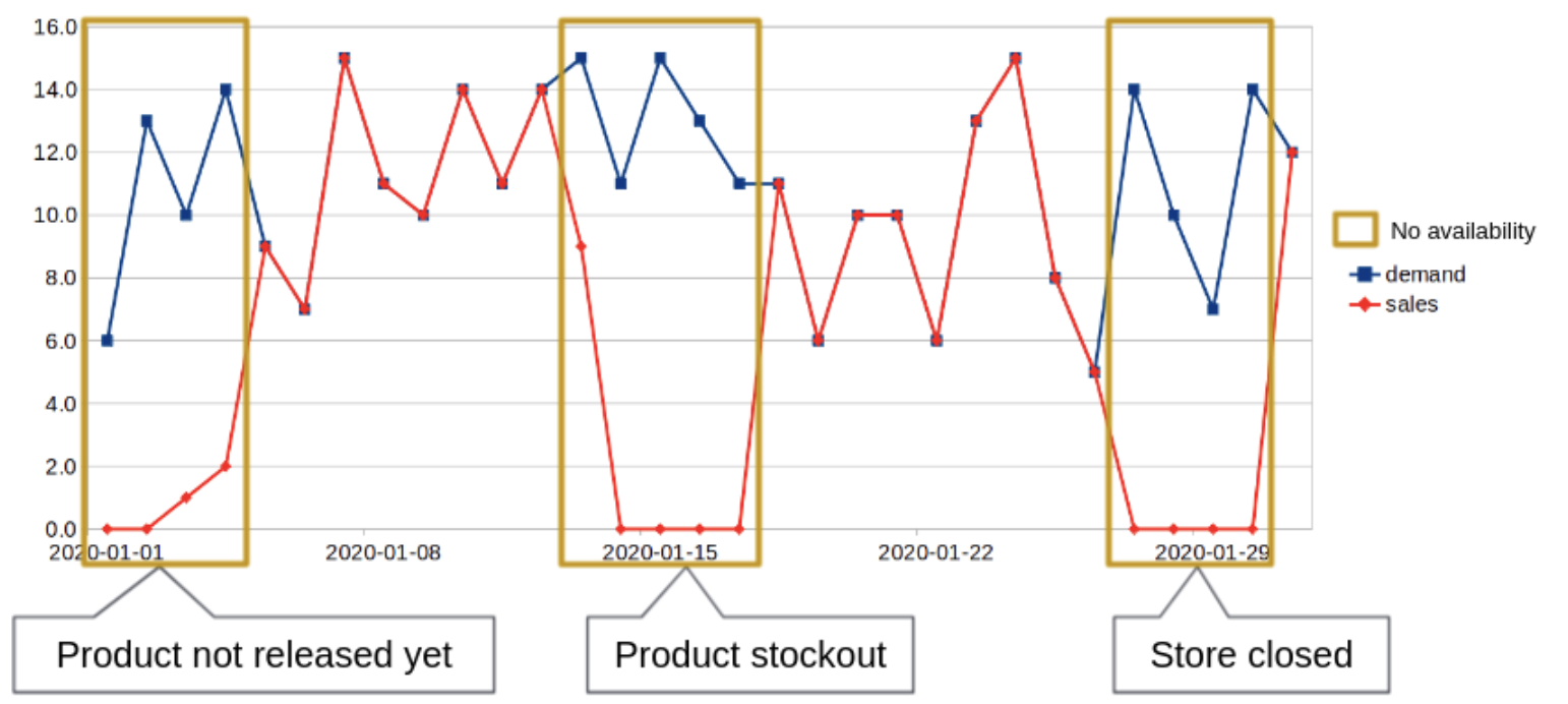
What is the difference?

• Demand is the amount we would sell if the store was open and stocked every day
• Sales are what actually happened, and are always lower or equal to demand

We will assume that Demand is equal to Sales when the product is available.

The past availability model covers following cases:

• Warehouse stockout (See below in the warehouse stockout section)
• First availability Date. The Product First Available Date is defined as the median of the first dates that the product is available in each store, thereby the product will be considered unavailable for all dates before the Product First Available Date. We use the median (that is similar to an average) as it is considered a more robust approach than a min or a max. 
• Store closing dates. A store is considered to have had a closing period if it has no sales for two or more consecutive days. All products are considered unavailable on a store when that store is on a closing period.

These three cases are the cases in which the historic data is considered not good to forecast the future, so it will be excluded. If these restrictions leave a product with less than 50% of days of availability (vs the number of weeks used as historic), stockout days starting from the beginning of the period will be used in the forecast until there are enough available days.

Warehouse stockout

In the long-term forecast (LTF) Stockout doesn't mean exactly 0 stock, since many times customers gradually become more conservative in replenishments so they don't get to 0 stock in WH in most cases. 

When a product is considered in stockout in the warehouse, the reorder solution will avoid using the sales data from those dates.

To assess whether a product is in WH stockout we apply several logics. 

Minimum quantity threshold: Is the amount of units of each product that need to be in the WH for the product to not be considered in stockout. Is measured as the relation between available units of a product in the WH with the amount of stores that need to be covered. This percentage is a parameter and currently is set to 10%. 

For example, if a product has 20 units in WH and it should be covering 300 stores (10% is 30), then these units are not considered enough and the product is in stockout.

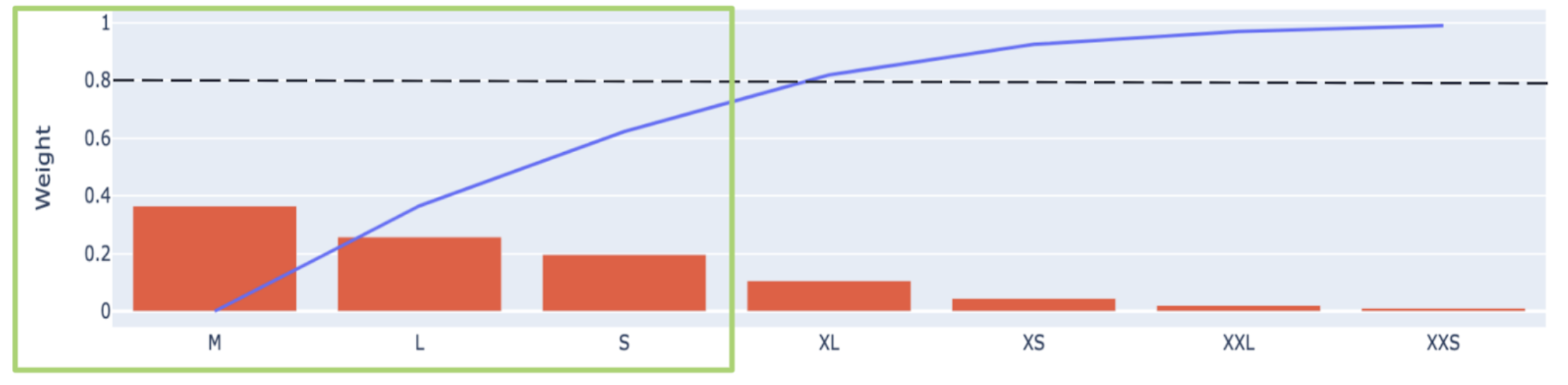
Size Curves for stockout: The sizes of a product don’t have all the same weight and importance within the product’s sales volume, we use size curves data to determine a good criteria for warehouse stockout and avoid residual sizes such as an XXXL can determine the stockout of the whole product.

To determine which sizes will be considered in the stockout criteria we select the top selling sizes that together sum more than the 80% of the whole volume of sales (at product level, not store level). The rest of the sizes are considered ‘irrelevant’ and will not be used to calculate stockout.

Corrected Stockout Dates

A product will need to be in stockout in WH during at least 10 days for it to be considered unavailable. After this, it will need to have 5 days of stock for it to be considered available again.

If these restrictions leave a product with less than 50% of days of availability (vs the number of weeks used as historic), stockout days starting from the beginning of the period will be used in the forecast until there are enough available days.

New stores / closing stores

Sometimes the sales perimeter changes during the lead time or coverage period, and we need to take those changes into account for the reorder suggestion. These are the main causes of the changes and how the algorithm takes them into account:

 

Opening of new stores (without previous history): In order to assign a correct weight to a new store and the products it has available, a relationship with a mirror store is assigned. The demand, the sales perimeter and the minimum stock are copied from this mirror store from the opening date to the end. On the day it opens, the store is initialized to maintain the minimum stock of all the skus in its sales perimeter (as long as there is stock in the warehouse).

 

Closing Store: Closing stores dates are taken into account when defining the past availability information, as mentioned, the closing of a store is marked when it has more than two consecutive days without any sales and it influences the availability of the products during those dates. For this case, the store closing demand is already set to 0 for the day they are closed according to the forecast. Additionally, there will be no minimum stock considerations for these stores. One last thing to consider is that the stock in those stores is kept "frozen" in those stores in the current version, meaning it is not made available again in the store network from the stock projection perspective.

Changes in layout

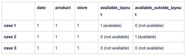
The are two main concepts that describe availability situation for a product-store combination:

• Inside store layout: When a product is present in a store and it is available for sale (what sometimes we mention as inside the selling perimeter).
• Outside store layout but still available for extraordinary sales: When a product is not in a store, but it is possible to order from other stores or from the warehouse (this could happen for example through store requests. Sometimes we describe this situation with the naming of “inside buying perimeter but outside selling perimeter).

There are three possible states for a store-product combination for a given date:

1. The product is present in the store, and can be bought in the store. The product is in the layout.
2. The product is not present in the store, but it can be ordered anyway sometimes. We still consider that sales could happen in this case, usually less often than inside the layout. The product is considered available but outside of the layout.
3. The product is not available in the store (either not being sold globally or the store is closed). This combination is never available in our forecast.

Availability Mask Structure. example

A product-store could change their availability status for one of these possible changes:

• Changes in the store layout (layout management), moving store-product combinations from being present in the store to not being present and vice-versa (between cases 1 and 2).
• Opening of new stores, replicating the demand of an existing store for all products (including the 2 previous changes).
• Closing of existing stores setting all store-product combinations on the dates that a store is closed to not available (not available at all, case 3).

All changes made to the availability status will be reflected in the Availability information for each product-store-date combination. In this way, our demand forecast algorithm will be taking into account the variations in the availability of the product-stores.

 

Future changes in the layout can be uploaded during the scenario configuration. 

These changes of course have an impact on the forecast. In each reorder scenario we calculate an average weight of the store (for all the products) both within sales occurring inside the layout and outside of the layout. Then for each change, the forecast will be increased/decreased in percentage using the weight of the store affected. 

Let’s imagine an example. The customer is launching a reorder scenario with 50 products and 100 stores. Within all the stores, store A used to not have reference 1 in the layout.

The customer has parametrized that starting from the beginning of the planning horizon, store A will have reference 1 in the layout. 
 

The solution calculates the weight that the store has in the sales both inside the layout and outside the layout (considering the total sales of that store within all the 50 products of the scenario).

The forecast is than adjusted considering that there will be an increment of the sales from stores with the product inside the layout (proportional to the weight of that store) and a decrease in the sales from the stores with that product outside of the layout.

Size curves

The size curve of a product is the relative weights that each of its sizes have. These weights are used to disaggregate our forecast from product-store-date level to sku-store-date level. The weight of each size is based on the volume sales share from the whole product’s sales. For example, on a sweater, a size M is more likely to have a greater volume of sales and therefore greater weight than an XXL size.

The pipeline will use as default the last year of sales to calculate this weights and generate size curves for the given products. Let’s illustrate with a simple example:

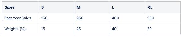
Product: Random sweater 101

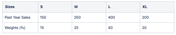
Following the example, if we have calculated a forecast of 700 skus for the same product and a certain time period, we will then distribute skus into sizes using previously calculated weights:

Forecasted sales: 700 SKUs

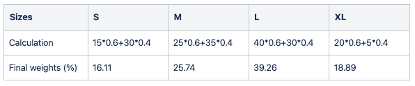
In order to grant robustness of the size curve, there’s a fallback depending on the sales volume of each product. When a product sales are under a threshold (200 by default) over the past defined period (1 year by default), aggregated sales at family level are taken into account for weights calculation. This fallback acts as a correction for weights instead of a substitution. Thus, final weight will be a proportion of product weight and product category weight as a linear ratio (product_sales/threshold). Let’s illustrate it:

Product: Bad seller sweater 102

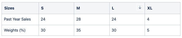
Total sales (product level): 80 SKUs

Threshold: 200 SKUs

Fallback into family category: Random sweaters

Weight ratio = Total sales / Threshold = 80/200 = 0.4 (40%)

Final weights for Bad seller sweater 102

final weight = fallback weight * (1-Weight ratio) + product weight * Weight ratio

This fallback will be applied recursively until threshold got satisfied. Thus, granting robustness.

All above explanations applies to the SizeCurveAutocomparablesPipeline which is being currently used.

The fallbacks used in reorder are product level, family level, normal distribution.

Product store weights

The weights of each product store combination are estimated to disaggregate our forecast demand from product level to product-store level. This is then used to calculate the stock projection at store level and therefore could have an impact in the final reorder proposal. The weight of each product-store is based on the volume and availiability sales share from the product in all stores.

Let’s illustrate with a simple example:

From Sales data we group the sales quantity by store-product.

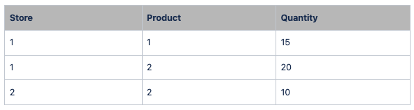
We estimate the mean of sales by store and estimate the weight of each store with respect to all available stores data.

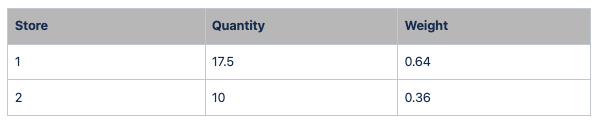
We assign the previous estimated weights by store to all products available in each store and multiply the availability of product, it means that when a product its not available in a store its weight will be 0.

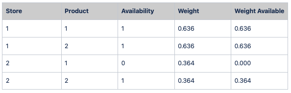
To estimate the real weight of each product-store we ponder the weight assigned (Weight Available) by the total weight available of each product in all the stores. For example for product 1 the total weight available is 0.636, since it was not available in store 2.

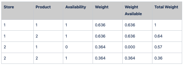
So in this example, the 100% of sales of product 1 corresponds to the sales in store 1 because it is in the only store where it is available.

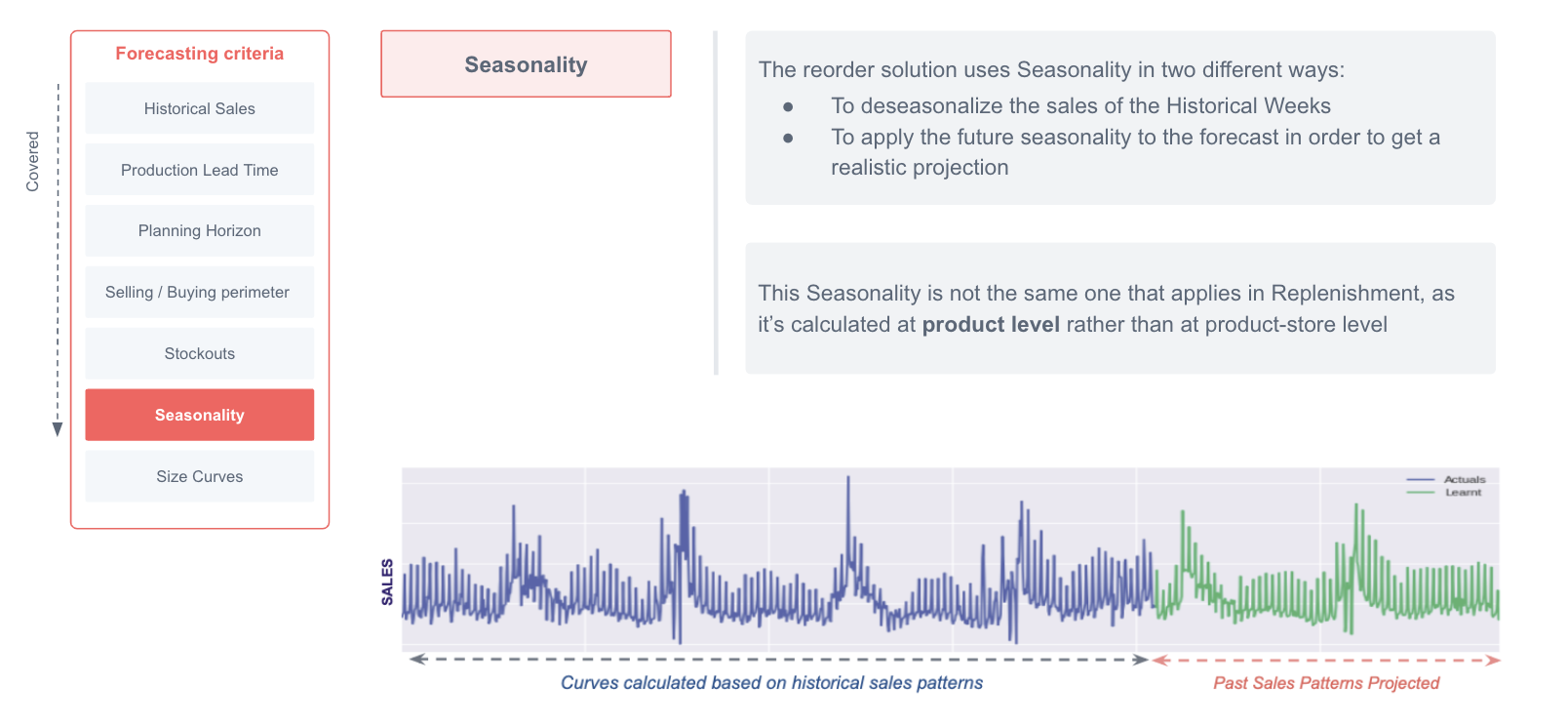
Seasonality

Seasonality is used in the long term forecast in the same way it is used in the short term forecast. This means that it is used to deseasonalize historic sales and then it is applied in the planning horizon period.  

The seasonality configuration is different from the one used in the short-term forecast as in reorder, we don't strictly need to have a granularity at store level (as we are interested in the general product forecast) and therefore the fallbacks level could differ.